Anscombe’s Quartet
Anscombe quartet emphasizes the need to move beyond basic numerical summaries of your data. The anscombe dataset has four sets of x and y variables with very similar summaries, but distinct visual patterns
Prep the data
anscombe## x1 x2 x3 x4 y1 y2 y3 y4
## 1 10 10 10 8 8.04 9.14 7.46 6.58
## 2 8 8 8 8 6.95 8.14 6.77 5.76
## 3 13 13 13 8 7.58 8.74 12.74 7.71
## 4 9 9 9 8 8.81 8.77 7.11 8.84
## 5 11 11 11 8 8.33 9.26 7.81 8.47
## 6 14 14 14 8 9.96 8.10 8.84 7.04
## 7 6 6 6 8 7.24 6.13 6.08 5.25
## 8 4 4 4 19 4.26 3.10 5.39 12.50
## 9 12 12 12 8 10.84 9.13 8.15 5.56
## 10 7 7 7 8 4.82 7.26 6.42 7.91
## 11 5 5 5 8 5.68 4.74 5.73 6.89First we’ll use tidyr to reshape the anscombe dataset to make it easier to work with. We want a column to identify each point, id, a column for the series (x1 is the x value in series 1), and columns for x and y. In the case of the anscombe dataset, rows group x and y vaules, but are not important across series.
library(tidyverse)
tidy_anscombe <- anscombe %>%
  mutate(id = row_number()) %>%
  gather(key = key, value = value, everything(), -id)
tidy_anscombe %>% as.tbl
## # A tibble: 88 x 3
## id key value
## <int> <chr> <dbl>
## 1 1 x1 10
## 2 2 x1 8
## 3 3 x1 13
## 4 4 x1 9
## 5 5 x1 11
## 6 6 x1 14
## 7 7 x1 6
## 8 8 x1 4
## 9 9 x1 12
## 10 10 x1 7
## # ... with 78 more rowsNow we want can split the key column into an x_or_y column and a series column.
tidy_anscombe <- tidy_anscombe %>%
  separate(key, c("x_or_y", "series"), 1)
tidy_anscombe %>% as.tbl
## # A tibble: 88 x 4
## id x_or_y series value
## * <int> <chr> <chr> <dbl>
## 1 1 x 1 10
## 2 2 x 1 8
## 3 3 x 1 13
## 4 4 x 1 9
## 5 5 x 1 11
## 6 6 x 1 14
## 7 7 x 1 6
## 8 8 x 1 4
## 9 9 x 1 12
## 10 10 x 1 7
## # ... with 78 more rowsNow we can use spread() to create the final form of our table, regrouping the associated x and y values. We could have done something simpler since we knew there were only 4 series, but the code we used will work for an arbitrary number of series.
tidy_anscombe <- tidy_anscombe %>%
  spread(x_or_y, value)
tidy_anscombe %>% as.tbl
## # A tibble: 44 x 4
## id series x y
## * <int> <chr> <dbl> <dbl>
## 1 1 1 10 8.04
## 2 1 2 10 9.14
## 3 1 3 10 7.46
## 4 1 4 8 6.58
## 5 2 1 8 6.95
## 6 2 2 8 8.14
## 7 2 3 8 6.77
## 8 2 4 8 5.76
## 9 3 1 13 7.58
## 10 3 2 13 8.74
## # ... with 34 more rowsNumeric summary
tidy_anscombe %>%
  group_by(series) %>%
  summarise(
    mean_x = mean(x),
    mean_y = mean(y),
    sd_x = sd(x),
    sd_y = sd(y),
    cor = cor(x, y)
  )
## # A tibble: 4 x 6
## series mean_x mean_y sd_x sd_y cor
## <chr> <dbl> <dbl> <dbl> <dbl> <dbl>
## 1 1 9 7.500909 3.316625 2.031568 0.8164205
## 2 2 9 7.500909 3.316625 2.031657 0.8162365
## 3 3 9 7.500000 3.316625 2.030424 0.8162867
## 4 4 9 7.500909 3.316625 2.030579 0.8165214Visual summary
While the numeric summaries suggest very similar datasets, the visual summaries help identify the differences:
library(ggplot2)
tidy_anscombe %>%
  ggplot(aes(x, y)) +
  geom_point() +
  facet_wrap(~ series) +
  coord_fixed()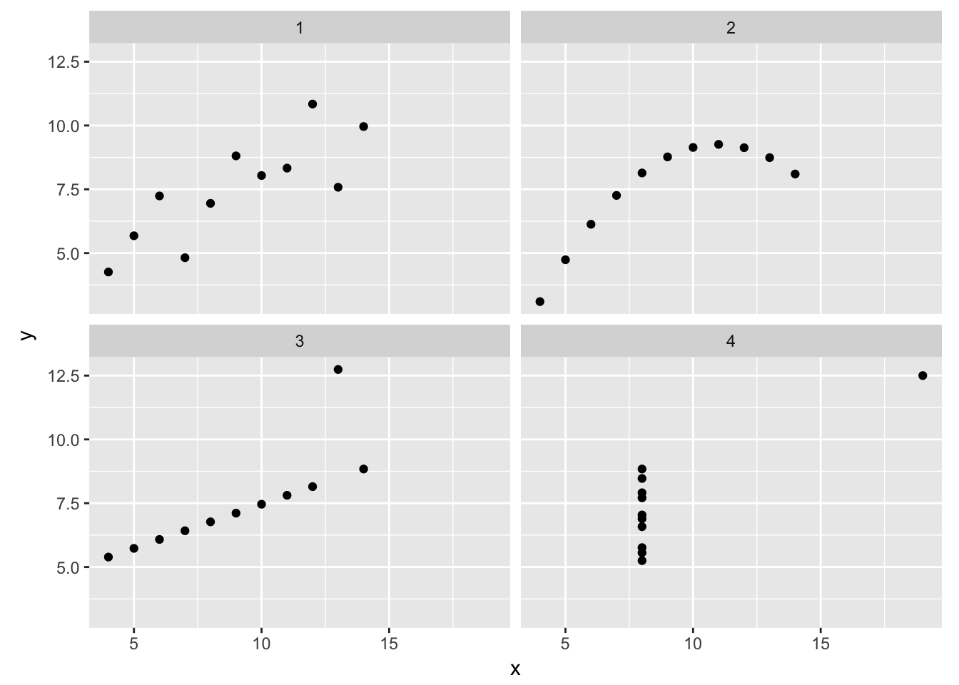
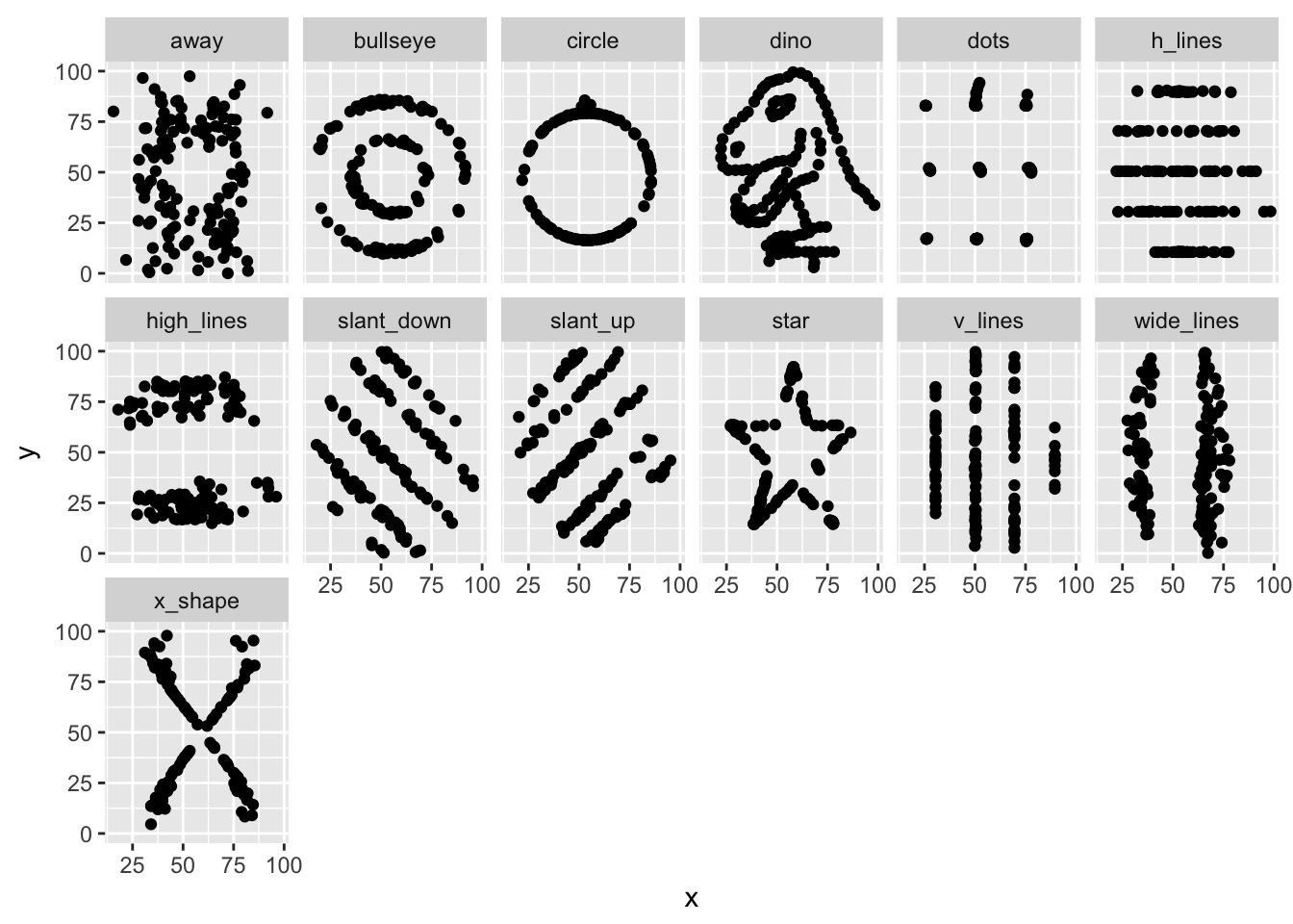
The Datasaurus Dozen
The Datasaurus Dozen is a set of series, like Anscombe’s quartet, with similar numerical summaries and radically different visual summaries. See a great discussion of this dataset by the creators, Justin Matejka and George Fitzmaurice here
Download the data here and move the DatasaurusDozen.tsv file into your data folder.
datasaurus <- read_tsv("data/DatasaurusDozen.tsv")
datasaurus %>%
  group_by(dataset) %>%
  summarise(
    mean_x = mean(x),
    mean_y = mean(y),
    sd_x = sd(x),
    sd_y = sd(y),
    cor = cor(x, y)
  )
## # A tibble: 13 x 6
## dataset mean_x mean_y sd_x sd_y cor
## <chr> <dbl> <dbl> <dbl> <dbl> <dbl>
## 1 away 54.26610 47.83472 16.76982 26.93974 -0.06412835
## 2 bullseye 54.26873 47.83082 16.76924 26.93573 -0.06858639
## 3 circle 54.26732 47.83772 16.76001 26.93004 -0.06834336
## 4 dino 54.26327 47.83225 16.76514 26.93540 -0.06447185
## 5 dots 54.26030 47.83983 16.76774 26.93019 -0.06034144
## 6 h_lines 54.26144 47.83025 16.76590 26.93988 -0.06171484
## 7 high_lines 54.26881 47.83545 16.76670 26.94000 -0.06850422
## 8 slant_down 54.26785 47.83590 16.76676 26.93610 -0.06897974
## 9 slant_up 54.26588 47.83150 16.76885 26.93861 -0.06860921
## 10 star 54.26734 47.83955 16.76896 26.93027 -0.06296110
## 11 v_lines 54.26993 47.83699 16.76996 26.93768 -0.06944557
## 12 wide_lines 54.26692 47.83160 16.77000 26.93790 -0.06657523
## 13 x_shape 54.26015 47.83972 16.76996 26.93000 -0.06558334Visual summaries
datasaurus %>%
  ggplot(aes(x, y)) +
  geom_point() +
  facet_wrap(~ dataset, ncol = 6) +
  coord_fixed()