Lecture 2 Reading data
The first step in analyzing data with R is reading data into it. This lesson focuses on reading data, manipulating it with dplyr and a few summary visualizations.
2.1 Data Source:
The US Census Bureau has a large selection of data on the population of the United States. The public-use micro surveys (PUMS) are available from the following link:
https://www.census.gov/programs-surveys/acs/data/pums.html
We’ll take a look at the 1-year American Community Survey results for the state of Hawaii.
The specific file we are working with is the person record, so not every variable in the data dictionary will be available. Only those under the heading “PERSON RECORD” will be in the csv_phi.zip file.
2.2 read_csv
To read in the downloaded file, we’ll use the readr package, which you can install by installing tidyverse.
library(tidyverse)
pop_hi <- read_csv("data/csv_phi.zip")
pop_hi
## # A tibble: 14,124 x 284
## RT SERIALNO SPORDER PUMA ST ADJINC PWGTP AGEP CIT CITWP
## <chr> <int> <chr> <chr> <int> <int> <chr> <chr> <int> <int>
## 1 P 21 01 00303 15 1001264 00078 63 1 NA
## 2 P 158 01 00306 15 1001264 00056 54 1 NA
## 3 P 267 01 00100 15 1001264 00059 52 5 NA
## 4 P 267 02 00100 15 1001264 00071 56 5 NA
## 5 P 267 03 00100 15 1001264 00102 25 5 NA
## 6 P 267 04 00100 15 1001264 00155 22 5 NA
## 7 P 267 05 00100 15 1001264 00074 15 5 NA
## 8 P 351 01 00100 15 1001264 00307 32 4 2005
## 9 P 351 02 00100 15 1001264 00578 02 1 NA
## 10 P 470 01 00200 15 1001264 00041 79 1 NA
## # ... with 14,114 more rows, and 274 more variables: COW <int>,
## # DDRS <int>, DEAR <int>, DEYE <int>, DOUT <int>, DPHY <int>,
## # DRAT <int>, DRATX <int>, DREM <int>, ENG <int>, FER <int>, GCL <int>,
## # GCM <int>, GCR <int>, HINS1 <int>, HINS2 <int>, HINS3 <int>,
## # HINS4 <int>, HINS5 <int>, HINS6 <int>, HINS7 <int>, INTP <chr>,
## # JWMNP <chr>, JWRIP <chr>, JWTR <chr>, LANX <int>, MAR <int>,
## # MARHD <int>, MARHM <int>, MARHT <int>, MARHW <int>, MARHYP <int>,
## # MIG <int>, MIL <int>, MLPA <int>, MLPB <int>, MLPCD <int>, MLPE <int>,
## # MLPFG <int>, MLPH <int>, MLPI <int>, MLPJ <int>, MLPK <int>,
## # NWAB <int>, NWAV <int>, NWLA <int>, NWLK <int>, NWRE <int>, OIP <chr>,
## # PAP <chr>, RELP <chr>, RETP <chr>, SCH <int>, SCHG <chr>, SCHL <chr>,
## # SEMP <chr>, SEX <int>, SSIP <chr>, SSP <chr>, WAGP <chr>, WKHP <chr>,
## # WKL <int>, WKW <int>, WRK <int>, YOEP <int>, ANC <int>, ANC1P <chr>,
## # ANC2P <chr>, DECADE <int>, DIS <int>, DRIVESP <int>, ESP <int>,
## # ESR <int>, FHICOVP <int>, FOD1P <int>, FOD2P <int>, HICOV <int>,
## # HISP <chr>, INDP <chr>, JWAP <chr>, JWDP <chr>, LANP <int>,
## # MIGPUMA <chr>, MIGSP <chr>, MSP <int>, NAICSP <chr>, NATIVITY <int>,
## # NOP <int>, OC <int>, OCCP <chr>, PAOC <int>, PERNP <chr>, PINCP <chr>,
## # POBP <chr>, POVPIP <chr>, POWPUMA <chr>, POWSP <chr>, PRIVCOV <int>,
## # PUBCOV <int>, QTRBIR <int>, ...2.3 dplyr
Using the data dictionary we can identify some interesting variables.
PERSON RECORD

RT      1
    Record Type
        P .Person Record

AGEP        2
    Age
        00  .Under 1 year
        01..99  .1 to 99 years (Top-coded***)

COW     1
    Class of worker
        b .N/A (less than 16 years old/NILF who last
          .worked more than 5 years ago or never worked)
        1 .Employee of a private for-profit company or
          .business, or of an individual, for wages,
          .salary, or commissions
        2 .Employee of a private not-for-profit,
          .tax-exempt, or charitable organization
        3 .Local government employee (city, county, etc.)
        4 .State government employee
        5 .Federal government employee
        6 .Self-employed in own not incorporated
          .business, professional practice, or farm
        7 .Self-employed in own incorporated
          .business, professional practice or farm
        8 .Working without pay in family business or farm
        9 .Unemployed and last worked 5 years ago or earlier or never
                  .worked

SCHL        2
    Educational attainment
        bb .N/A (less than 3 years old)
        01 .No schooling completed
        02 .Nursery school, preschool
        03 .Kindergarten
        04 .Grade 1
        05 .Grade 2
        06 .Grade 3
        07 .Grade 4
        08 .Grade 5
        09 .Grade 6
        10 .Grade 7
        11 .Grade 8
        12 .Grade 9
        13 .Grade 10
        14 .Grade 11
        15 .12th grade - no diploma
        16 .Regular high school diploma
        17 .GED or alternative credential
        18 .Some college, but less than 1 year
        19 .1 or more years of college credit, no degree
        20 .Associate's degree
        21 .Bachelor's degree
        22 .Master's degree
        23 .Professional degree beyond a bachelor's degree
        24 .Doctorate degree

WAGP        6
    Wages or salary income past 12 months
        bbbbbb      .N/A (less than 15 years old)
        000000      .None
        000001..999999  .$1 to 999999 (Rounded and top-coded)

Note: Use ADJINC to adjust WAGP to constant dollars.


WKHP        2
    Usual hours worked per week past 12 months
        bb   .N/A (less than 16 years old/did not work
             .during the past 12 months)
        01..98   .1 to 98 usual hours
        99   .99 or more usual hours

WKW     1
    Weeks worked during past 12 months
        b .N/A (less than 16 years old/did not work
          .during the past 12 months)
        1 .50 to 52 weeks worked during past 12 months
        2 .48 to 49 weeks worked during past 12 months
        3 .40 to 47 weeks worked during past 12 months
        4 .27 to 39 weeks worked during past 12 months
        5 .14 to 26 weeks worked during past 12 months
        6 .less than 14 weeks worked during past 12 months

ESR     1
    Employment status recode
        b .N/A (less than 16 years old)
        1 .Civilian employed, at work
        2 .Civilian employed, with a job but not at work
        3 .Unemployed
        4 .Armed forces, at work
        5 .Armed forces, with a job but not at work
        6 .Not in labor force

PERNP       7
    Total person's earnings
        bbbbbbb         .N/A (less than 15 years old)
        0000000         .No earnings
        -010000         .Loss of $10000 or more (Rounded & bottom-coded
                        .components)
        -000001..-009999    .Loss $1 to $9999 (Rounded components)
        0000001         .$1 or break even
        0000002..9999999    .$2 to $9999999 (Rounded & top-coded components)

Note: Use ADJINC to adjust PERNP to constant dollars.

PINCP       7
    Total person's income (signed)
        bbbbbbb         .N/A (less than 15 years old)
        0000000         .None
        -019999         .Loss of $19999 or more (Rounded & bottom-coded
                        .components)
        -000001..-019998    .Loss $1 to $19998 (Rounded components)
        0000001         .$1 or break even
        0000002..9999999    .$2 to $9999999 (Rounded & top-coded components)

Note: Use ADJINC to adjust PINCP to constant dollars.
Let’s focus on employed civilians (ESR either 1 or 2) working full time (WKHP > 32) for close to the entire year (WKW either 1 or 2).
pop_hi <- pop_hi %>%
  filter(
    ESR %in% c(1, 2),
    as.numeric(WKHP) > 32,
    WKW %in% c(1, 2)
  )
If you are unsure if a column that you want to treat as numeric contains letters, you can run the following command to get a list of the values containing letters:
grep("[[:alpha:]]", pop_hi$WKHP, value = TRUE)## character(0)We can use two functions to add new columns (or change existing ones).
mutate()adds columns and keeps the previous columnstransmute()adds columns and removes the previous columns
This time we want to drop the columns we don’t mention.
pop_hi <- pop_hi %>%
  transmute(
    age = as.numeric(AGEP),
    worker_class = factor(COW, labels = c(
      "for-profit",
      "not-for-profit",
      "local government",
      "state government",
      "federal government",
      "self-employed not incorporated",
      "self-employed incorporated",
      "family business no pay"
    )),
    school = SCHL,
    wages = as.numeric(WAGP),
    top_coded_wages = WAGP == 999999
)
Creating a custom factor variable for educational attainment:
education_levels <- c("less than HS", "HS", "associates", "bachelors", "masters", "doctorate")

pop_hi$education <- NA
pop_hi[pop_hi$school < 16,]$education <- "less than HS"
pop_hi[pop_hi$school > 16 & pop_hi$school < 20,]$education <- "HS"
pop_hi[pop_hi$school == 20,]$education <- "associates"
pop_hi[pop_hi$school == 21,]$education <- "bachelors"
pop_hi[pop_hi$school %in% c(22, 23),]$education <- "masters"
pop_hi[pop_hi$school == 24,]$education <- "doctorate"

pop_hi <- pop_hi %>%
  mutate(education = factor(education, levels = education_levels))
2.4 First Look at ggplot2
See the ggplot2 documentation for details and inspiration.
ggplot(pop_hi, aes(age, wages)) +
  geom_point()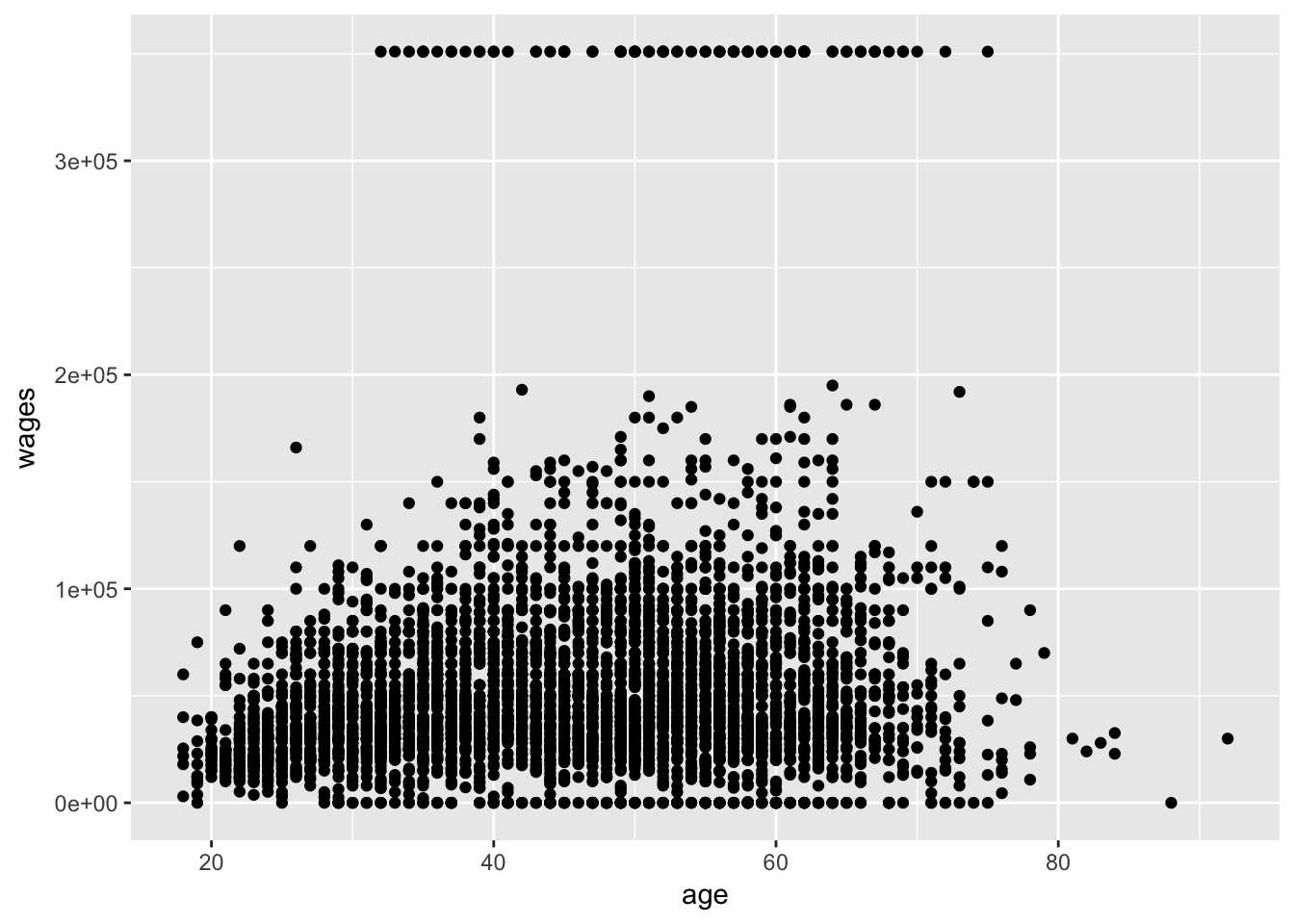
Income has a skewed distribution, so it is often presented/analyzed in logs. Here’s how to modify the above chart to display income in logs:
pop_hi <- pop_hi %>%
  mutate(log_safe_wages = ifelse(wages == 0, 1, wages))
pop_hi %>%
  ggplot(aes(age, log_safe_wages)) +
  geom_point() +
  scale_y_log10()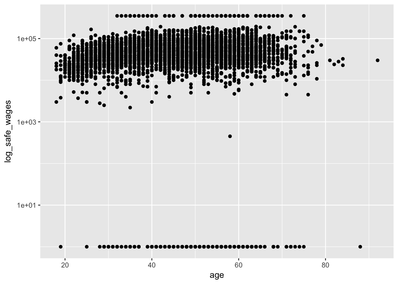
2.5 Heatmaps
Heatmaps allow you to get a sense of the concetration of observations in regions where there are many overlapping points:
ggplot(pop_hi, aes(age, log_safe_wages)) +
  geom_bin2d() +
  scale_y_log10()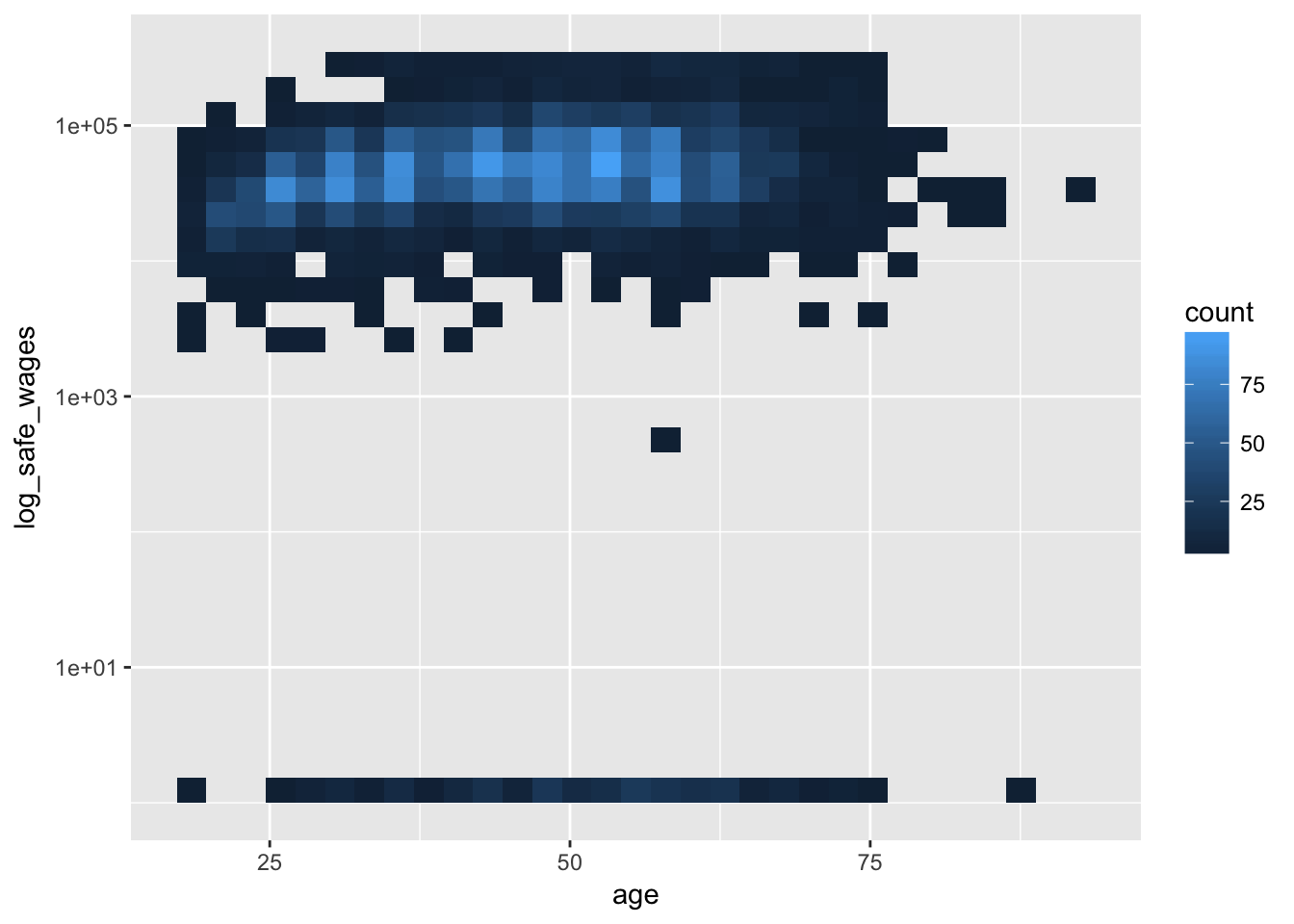
2.6 Hexbins
Hexbins use hexagons instead of squares, which helps avoid the rectangular sections in heatmaps that may misrepresent your data.
You will need to install the hexbin package.
install.packages("hexbin")pop_hi %>%
filter(wages > 10000, wages < 300000) %>%
ggplot(aes(age, wages)) +
geom_hex() +
scale_x_log10()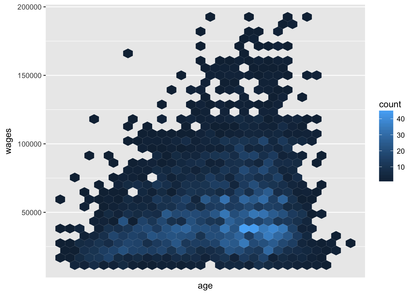
Here we can see that inequality in wages for workers increases with age.
2.7 Other topics from this dataset
This dataset includes information on the majors for degree holders and the industry codes. You could use that additional information to ask how well targeted majors are to particular industries and how incomes vary across choice of major. Because of the size of the data in the Hawaii sample, it would be better to ask some of these questions at the national level.
Go to the ACS PUMS documentation page for more information.
2.8 Assignment
Choose another pair of variables from the data dictionary and visualize them with a scatterplot, a heatmap, and a hexbin plot.