Lecture 16 Time-Series Modeling
This lecture uses the following packages:
tidyverse
tidyquant
vars
16.1 Introduction
The focus of this lecture is on time-series data. We will be making use of a new package that helps us apply the tools of the tidyverse to time series. To read more about the tidyquant package, check out its website:
16.2 Data
To explore time-series modeling, we will download a few macroeconomic time series from
FRED. The data list I compiled for this lecture can be accessed at the following link:
https://research.stlouisfed.org/pdl/988
The following steps assume you used the Zipped Tab Delimted Text option with 1972-01-01 as the start date.
library(tidyverse)

daily <- read_tsv(
  "data/Time_series_lecture_txt/Time_series_lecture_Daily.txt",
  na = c(".")
)
monthly <- read_tsv(
  "data/Time_series_lecture_txt/Time_series_lecture_Monthly.txt",
  na = c(".")
)
quarterly <- read_tsv(
  "data/Time_series_lecture_txt/Time_series_lecture_Quarterly.txt",
  na = c(".")
) %>%
  mutate(GDPC1_CHG = c(NA, diff(GDPC1)))
Since we have data in multiple frequencies, we first need to aggregate up to the quarterly level.
library(tidyquant)
daily_q <- daily %>%
  tq_transmute(mutate_fun = to.quarterly)
monthly_q <- monthly %>%
  tq_transmute(mutate_fun = to.quarterly)
all_q <- quarterly %>%
  mutate(DATE = as.yearqtr(DATE, format = "%Y-%m-%d")) %>%
  merge(monthly_q, all = TRUE) %>%
  merge(daily_q, all = TRUE)
head(all_q)
## DATE CBIC1 GDPC1 GDPC1_CHG EMRATIO HOUST IPMANSICS PERMIT USTRADE
## 1 1972 Q1 12.299 5002.436 NA 56.9 2334 39.4883 2105 7946.6
## 2 1972 Q2 40.281 5118.278 115.842 57.0 2254 40.1413 2183 8019.4
## 3 1972 Q3 43.105 5165.448 47.170 57.0 2481 40.9834 2393 8073.1
## 4 1972 Q4 17.313 5251.226 85.778 57.3 2366 42.6782 2419 8224.1
## 5 1973 Q1 28.392 5380.502 129.276 57.8 2365 43.7572 2062 8306.8
## 6 1973 Q2 55.489 5441.504 61.002 58.0 2067 43.9351 2051 8370.6
## NASDAQCOM
## 1 128.14
## 2 130.08
## 3 129.61
## 4 133.73
## 5 117.46
## 6 100.9816.3 Hold-Out Set
Just like in the previous lecture we want to use a training set so that we can evaluate the accuracy of our model on new data. In the context of time-series data, the validation/test sets are usually referred to as the hold-out set.
train <- all_q %>% filter(DATE < "2010 Q1")
hold_out <- all_q %>% filter(DATE >= "2010 Q1")
16.4 GDP
Let’s begin by plotting the series we want to predict (GDP):
ggplot(train, aes(x = DATE, y = GDPC1)) +
  geom_line() +
  scale_x_yearqtr() +
  labs(title = "Real GDP")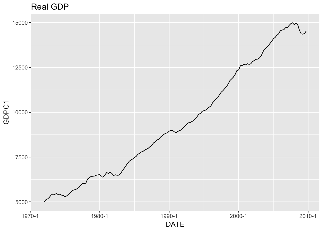
The GDP series in not stationary (you can see that the mean changes over time). Let’s look at GDPC1_CHG, which is real GDP change from one quarter to the next.
ggplot(train) +
  geom_line(aes(DATE, GDPC1_CHG)) +
  scale_x_yearqtr() +
  labs(title = "Real GDP Change")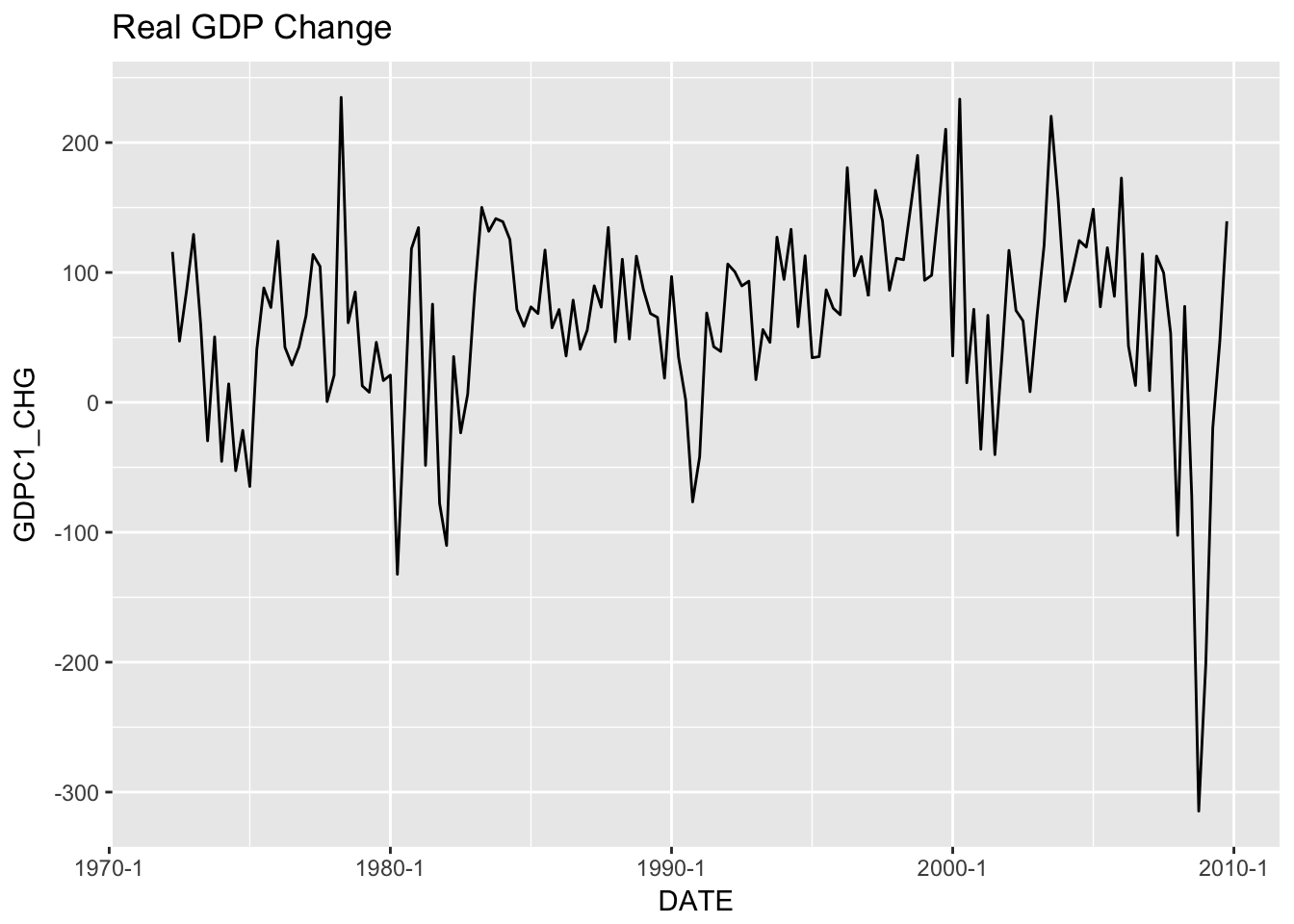
This series appears stationary so we’ll use it when the model we look at requires a stationary series.
16.5 Autoregressive Model
The Autoregressive (AR) model says that previous values are our best predictors of the future.
Here is the equation for an AR(1) model:
\[ y_t = \rho y_{t-1} + \varepsilon_t \]
\(y_{t-1}\) is the value last period.
There are many options possible with the ar() function, but we will stick to the defaults.
ar_model <- ar(train$GDPC1_CHG, na.action = na.omit)
ar_model
##
## Call:
## ar(x = train$GDPC1_CHG, na.action = na.omit)
##
## Coefficients:
## 1 2
## 0.3734 0.1465
##
## Order selected 2 sigma^2 estimated as 460616.5.1 AR Performance
ar_prediction <- predict(ar_model, newdata = c(0), n.ahead = 12)
ar_prediction
## $pred
## Time Series:
## Start = 2
## End = 13
## Frequency = 1
## [1] 30.33208 41.65808 50.33007 55.22716 58.32595 60.20034 61.35413
## [8] 62.05950 62.49189 62.75666 62.91886 63.01821
##
## $se
## Time Series:
## Start = 2
## End = 13
## Frequency = 1
## [1] 67.86826 72.44526 74.99879 75.79498 76.11146 76.22692 76.27062
## [8] 76.28695 76.29309 76.29539 76.29625 76.29657ggplot(cbind(hold_out[1:12,c("DATE", "GDPC1_CHG")], as.data.frame(ar_prediction)), aes(x = DATE)) +
geom_ribbon(aes(ymin = pred - se, ymax = pred + se), alpha = 0.25, fill = scales::muted("green")) +
geom_line(aes(y = pred), lty = 2) +
geom_line(aes(y = GDPC1_CHG)) +
scale_x_yearqtr() +
scale_y_continuous() +
labs(title = "AR prediction of GDP Change", subtitle = "Actual = solid, prediciton = dashed, se = green")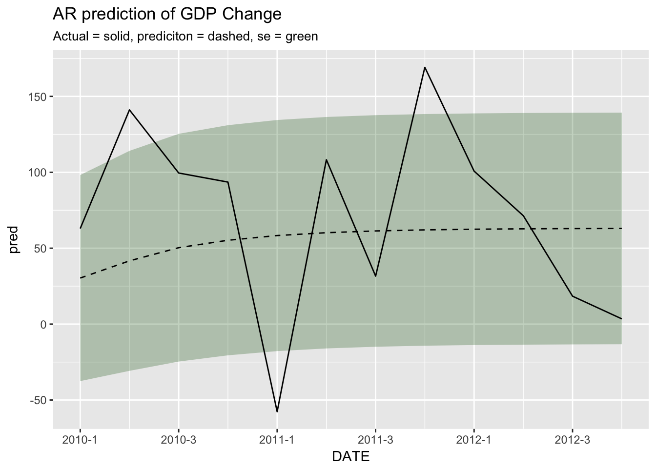
16.6 ARIMA
An Autoregressive integrated moving average (ARIMA) model is able to model non-stationary series. Just like the ar() function, the arima() function has many options for tuning the results. Again we will stick to the defaults, but we do need to specify the order parameter. The order is a three integer vector, (p, d, q), where p is the autoregressive order (above we had 2), d is the degree of differecing (we implicitly assumed this to be 1), and q is the moving average order. Since ARIMA can handle non-stationary series we will model GDPC1.
arima_model <- arima(train$GDPC1, c(2, 1, 0))
arima_model
##
## Call:
## arima(x = train$GDPC1, order = c(2, 1, 0))
##
## Coefficients:
## ar1 ar2
## 0.4951 0.2622
## s.e. 0.0789 0.0789
##
## sigma^2 estimated as 4998: log likelihood = -857.64, aic = 1721.2816.6.1 ARIMA Performance
arima_prediction <- predict(arima_model, n.ahead = 12)
arima_prediction
## $pred
## Time Series:
## Start = 153
## End = 164
## Frequency = 1
## [1] 14623.23 14700.05 14759.41 14808.94 14849.02 14881.85 14908.62
## [8] 14930.48 14948.31 14962.88 14974.76 14984.47
##
## $se
## Time Series:
## Start = 153
## End = 164
## Frequency = 1
## [1] 70.69357 127.15697 190.28257 254.15813 318.06299 380.88473 442.16208
## [8] 501.58832 559.02786 614.43429 667.82451 719.25352We can compare the ARIMA prediction to the actual values.
ggplot(cbind(hold_out[1:12,c("DATE", "GDPC1")], as.data.frame(arima_prediction)), aes(x = DATE)) +
  geom_ribbon(aes(ymin = pred - se, ymax = pred + se), alpha = 0.25, fill = scales::muted("green")) +
  geom_line(aes(y = pred), lty = 2) +
  geom_line(aes(y = GDPC1)) +
  scale_x_yearqtr() +
  scale_y_continuous() +
  labs(title = "ARIMA prediction of GDP", subtitle = "Actual = solid, prediciton = dashed, se = green")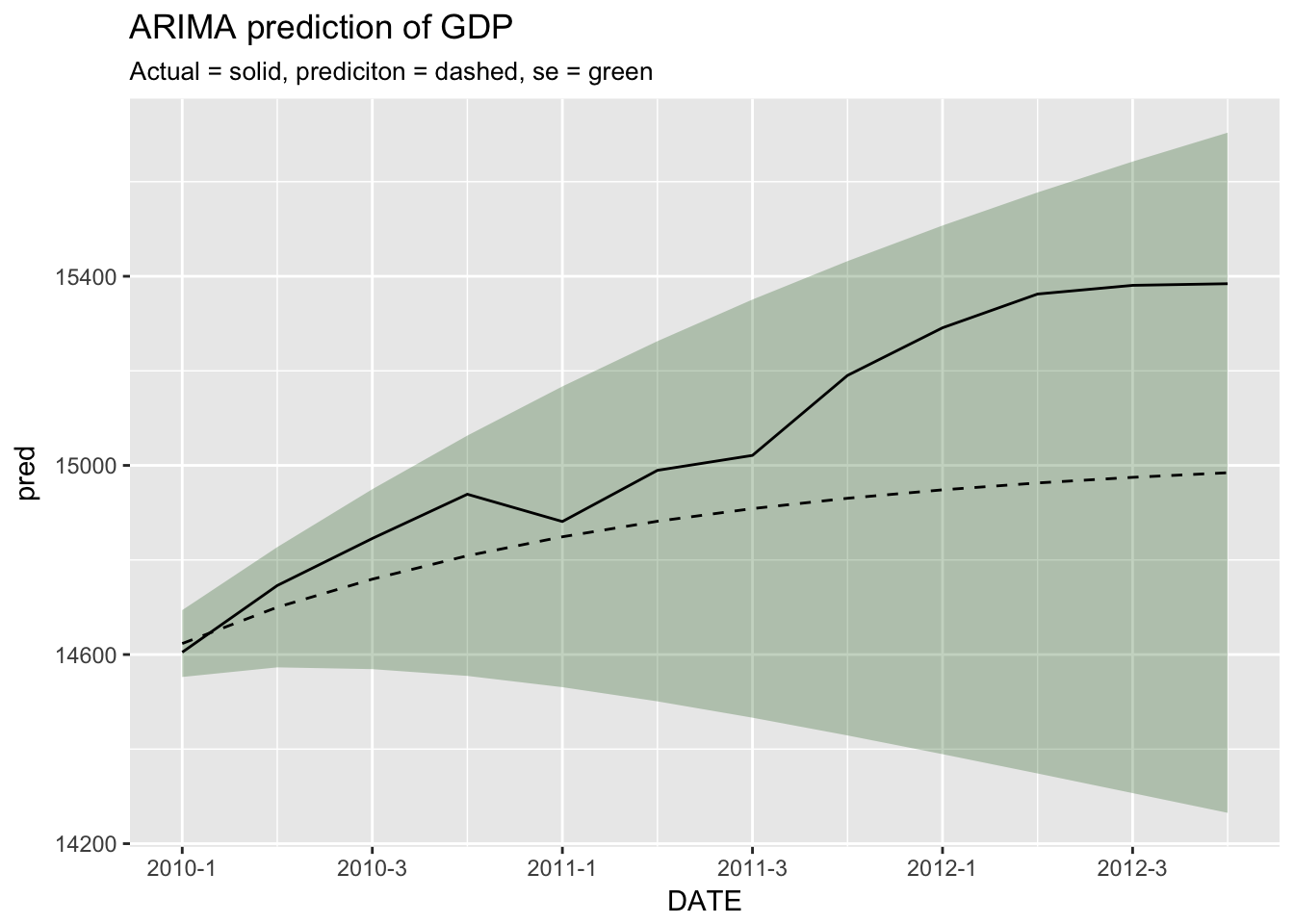
16.7 Vector Autoregression
Another approach is using a system of variables and allowing old values of each variable to affect the others.
library(vars)
var_model <- VAR(train %>% dplyr::select(GDPC1, CBIC1, PERMIT), p = 2)
var_model
##
## VAR Estimation Results:
## =======================
##
## Estimated coefficients for equation GDPC1:
## ==========================================
## Call:
## GDPC1 = GDPC1.l1 + CBIC1.l1 + PERMIT.l1 + GDPC1.l2 + CBIC1.l2 + PERMIT.l2 + const
##
## GDPC1.l1 CBIC1.l1 PERMIT.l1 GDPC1.l2 CBIC1.l2
## 1.43580900 -0.58917688 0.11891599 -0.43578050 0.41277606
## PERMIT.l2 const
## -0.07028366 -31.27177629
##
##
## Estimated coefficients for equation CBIC1:
## ==========================================
## Call:
## CBIC1 = GDPC1.l1 + CBIC1.l1 + PERMIT.l1 + GDPC1.l2 + CBIC1.l2 + PERMIT.l2 + const
##
## GDPC1.l1 CBIC1.l1 PERMIT.l1 GDPC1.l2 CBIC1.l2
## 0.27499817 0.26622923 -0.01514752 -0.27662607 0.25766133
## PERMIT.l2 const
## 0.02982024 -11.41669980
##
##
## Estimated coefficients for equation PERMIT:
## ===========================================
## Call:
## PERMIT = GDPC1.l1 + CBIC1.l1 + PERMIT.l1 + GDPC1.l2 + CBIC1.l2 + PERMIT.l2 + const
##
## GDPC1.l1 CBIC1.l1 PERMIT.l1 GDPC1.l2 CBIC1.l2
## -0.09626649 0.50352114 1.02625655 0.09599222 -0.38516155
## PERMIT.l2 const
## -0.10390036 111.02122210var_prediction <- predict(var_model, n.ahead = 12)
var_prediction## $GDPC1
## fcst lower upper CI
## [1,] 14552.09 14428.14 14676.04 123.9503
## [2,] 14581.90 14362.44 14801.37 219.4656
## [3,] 14614.81 14316.20 14913.41 298.6046
## [4,] 14647.63 14279.68 15015.57 367.9448
## [5,] 14682.57 14250.80 15114.34 431.7711
## [6,] 14719.60 14227.66 15211.54 491.9397
## [7,] 14758.43 14208.98 15307.88 549.4520
## [8,] 14798.94 14194.01 15403.87 604.9275
## [9,] 14840.98 14182.23 15499.73 658.7516
## [10,] 14884.42 14173.25 15595.59 711.1726
## [11,] 14929.15 14166.79 15691.51 762.3579
## [12,] 14975.05 14162.63 15787.48 812.4249
##
## $CBIC1
## fcst lower upper CI
## [1,] -54.72311 -113.4161 3.969862 58.69298
## [2,] -51.43549 -123.9368 21.065856 72.50135
## [3,] -44.19701 -124.3483 35.954254 80.15126
## [4,] -39.78960 -124.6068 45.027623 84.81723
## [5,] -36.19733 -124.0671 51.672487 87.86982
## [6,] -32.94117 -123.0147 57.132343 90.07351
## [7,] -30.06393 -121.8203 61.692405 91.75633
## [8,] -27.50770 -120.5942 65.578797 93.08650
## [9,] -25.21998 -119.3806 68.940582 94.16057
## [10,] -23.16746 -118.2047 71.869752 95.03721
## [11,] -21.32295 -117.0791 74.433163 95.75611
## [12,] -19.66354 -116.0101 76.683031 96.34657
##
## $PERMIT
## fcst lower upper CI
## [1,] 766.2323 479.0121 1053.453 287.2203
## [2,] 814.9529 407.6930 1222.213 407.2598
## [3,] 856.0776 369.8733 1342.282 486.2042
## [4,] 895.2920 349.9675 1440.617 545.3246
## [5,] 930.6943 340.0841 1521.304 590.6101
## [6,] 962.8492 336.8620 1588.836 625.9872
## [7,] 992.2160 338.1076 1646.324 654.1084
## [8,] 1019.0231 342.3067 1695.740 676.7164
## [9,] 1043.4904 348.4537 1738.527 695.0366
## [10,] 1065.8233 355.8536 1775.793 709.9698
## [11,] 1086.2063 364.0110 1808.402 722.1953
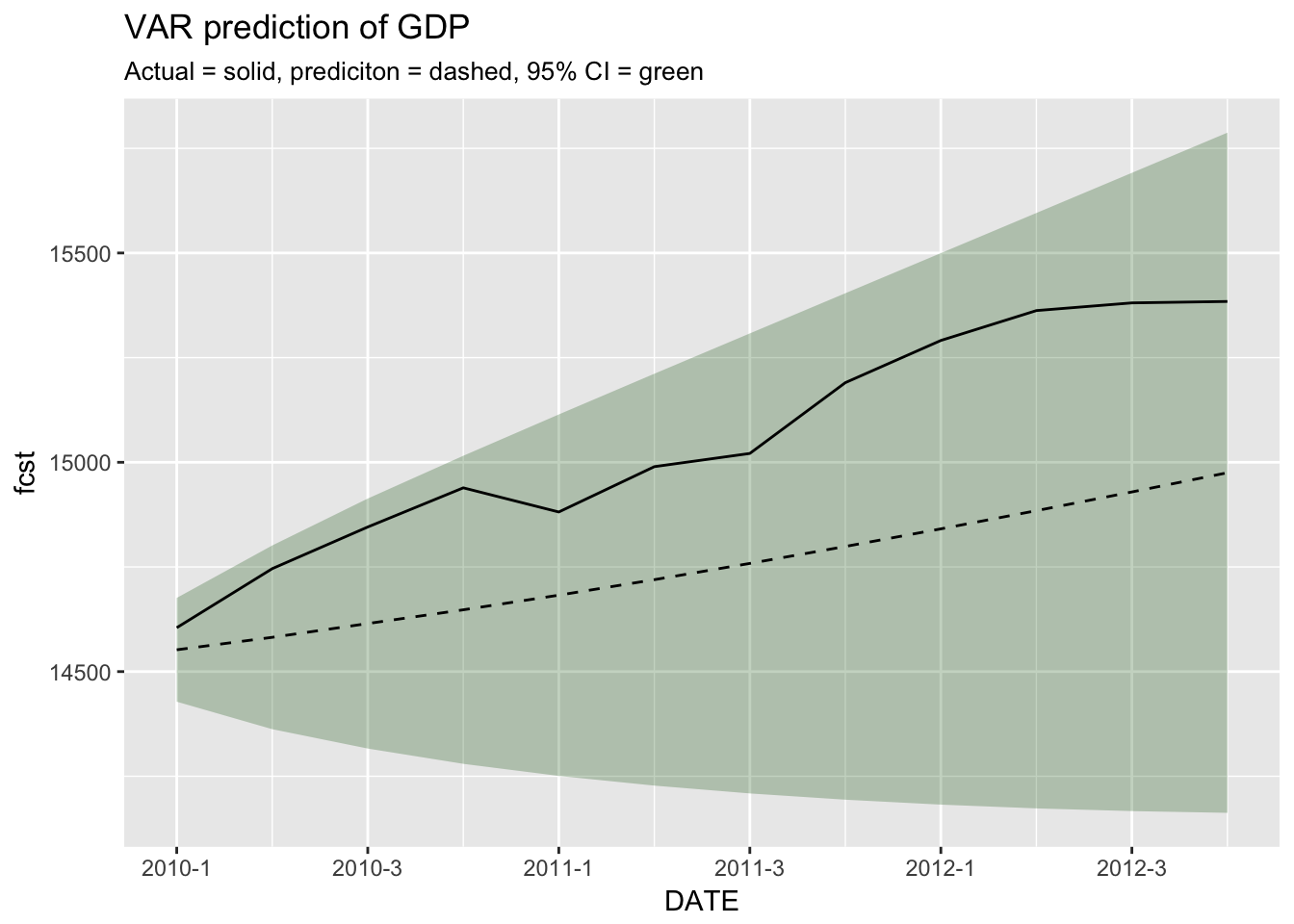
## [12,] 1104.8068 372.5697 1837.044 732.2371ggplot(
cbind(hold_out[1:12,c("DATE", "GDPC1")], as.data.frame(var_prediction$fcst$GDPC1)),
aes(x = DATE)
) +
geom_ribbon(aes(ymin = lower, ymax = upper), alpha = 0.25, fill = scales::muted("green")) +
geom_line(aes(y = fcst), lty = 2) +
geom_line(aes(y = GDPC1)) +
scale_x_yearqtr() +
scale_y_continuous() +
labs(
title = "VAR prediction of GDP",
subtitle = "Actual = solid, prediciton = dashed, 95% CI = green"
)
16.8 Assignment
Pick your preferred model and test its performance in the entire hold-out dataset. Report the RMSE (see the previous lesson) and create a chart like the ones above showing lines for the actual and predicted values with a blue ribbon indicating one standard error (for AR or ARIME) or the confidence interval (for VAR) about the prediciton.