Lecture 11 Polar Coordinates
This lecture uses the following packages:
tidyverse
lubridate
forcats
11.1 Data
Survey of Consumers
The University of Michigan conducts the Survey of Consumers. This monthly survey takes the pulse of consumers to help predict the state of the economy in the near future. We will be using a few responses from this monthly survey to highlight how you can visualize periodic data. For full definitions of the variables we will work with take a look at the online codebook: https://data.sca.isr.umich.edu/subset/codebook.php
To download the data
- Go to the Survey of Consumers’ data page: https://data.sca.isr.umich.edu/subset/subset.php
- In the Frequency and Range section, set the Starting year to 1998, since that is the first year with complete data on “Probability of Losing a Job During the Next 5 Years” (PJOB)
- In the Demographics section, check all Income groups (y13 = Bottom 33%, y23 = Middle 33%, and y33 = Top 33%)
- In the Variables section, check PEXP and PJOB in the Personal Finances subsection, and check UMEX in the Unemployment, Interest Rates, Prices, Government Expectations subsection
- Click on the “Download CSV” button.
Load the downloaded dataset.
library(tidyverse)
survey <- read_csv("data/scaum-814.csv")
Divide the date column into year and month columns.
library(lubridate)
survey <- survey %>%
  mutate(date = parse_date(yyyymm, format = "%Y%m"),
         year = year(date),
         month = month(date)
  ) %>%
  select(-yyyymm)
survey
## # A tibble: 235 x 12
## pexp_r_y13 pexp_r_y23 pexp_r_y33 pjob_mean_y13 pjob_mean_y23
## <int> <int> <int> <dbl> <dbl>
## 1 128 153 148 15.3 16.6
## 2 147 143 149 18.9 19.8
## 3 125 141 137 14.4 16.4
## 4 133 134 149 14.2 18.5
## 5 126 129 150 15.8 16.8
## 6 128 139 137 14.4 14.8
## 7 132 142 146 17.0 18.6
## 8 131 143 145 15.8 19.3
## 9 126 135 135 18.1 17.2
## 10 132 134 136 19.4 16.6
## # ... with 225 more rows, and 7 more variables: pjob_mean_y33 <dbl>,
## # umex_r_y13 <int>, umex_r_y23 <int>, umex_r_y33 <int>, date <date>,
## # year <dbl>, month <dbl>Each variable is calculated from the survey as follows:
| Code | Survey Question | Calculation |
|---|---|---|
| PEXP | “Now looking ahead – do you think that a year from now you (and your family living there) will be better off financially, worse off, or just about the same as now?” | Better - Worse + 100 |
| PJOB | “During the next 5 years, what do you think the chances are that you (or your husband/wife) will lose a job you wanted to keep?” | Mean |
| UMEX | “How about people out of work during the coming 12 months ‐‐ do you think that there will be more unemployment than now, about the same, or less?” | Less - More + 100 |
To make our dataset tidy, we want each variable to have it’s own row. Since we added the income demographic option, we have multiple columns for each variable. Let’s fix that with the gather() -> separate() -> spread() pattern.
library(forcats)
survey <- survey %>%
  gather(key = "key", value = "value", -year, -month, -date) %>%
  separate(key, into = c("variable", "type", "income")) %>%
  select(-type) %>%
  spread(key = "variable", value = "value") %>%
  mutate(income = fct_recode(as_factor(income), `Bottom 3rd` = "y13", `Middle 3rd` = "y23", `Top 3rd` = "y33"))
survey
## # A tibble: 705 x 7
## date year month income pexp pjob umex
## <date> <dbl> <dbl> <fctr> <dbl> <dbl> <dbl>
## 1 1998-01-01 1998 1 Bottom 3rd 128 15.3 90
## 2 1998-01-01 1998 1 Middle 3rd 153 16.6 94
## 3 1998-01-01 1998 1 Top 3rd 148 15.8 99
## 4 1998-02-01 1998 2 Bottom 3rd 147 18.9 103
## 5 1998-02-01 1998 2 Middle 3rd 143 19.8 103
## 6 1998-02-01 1998 2 Top 3rd 149 14.7 100
## 7 1998-03-01 1998 3 Bottom 3rd 125 14.4 90
## 8 1998-03-01 1998 3 Middle 3rd 141 16.4 106
## 9 1998-03-01 1998 3 Top 3rd 137 17.8 104
## 10 1998-04-01 1998 4 Bottom 3rd 133 14.2 101
## # ... with 695 more rows11.2 Simple Time Series
ggplot(survey, aes(date, pexp, color = income)) +
  geom_line() +
  geom_hline(yintercept = 100) +
  ggtitle("Better or Worse?")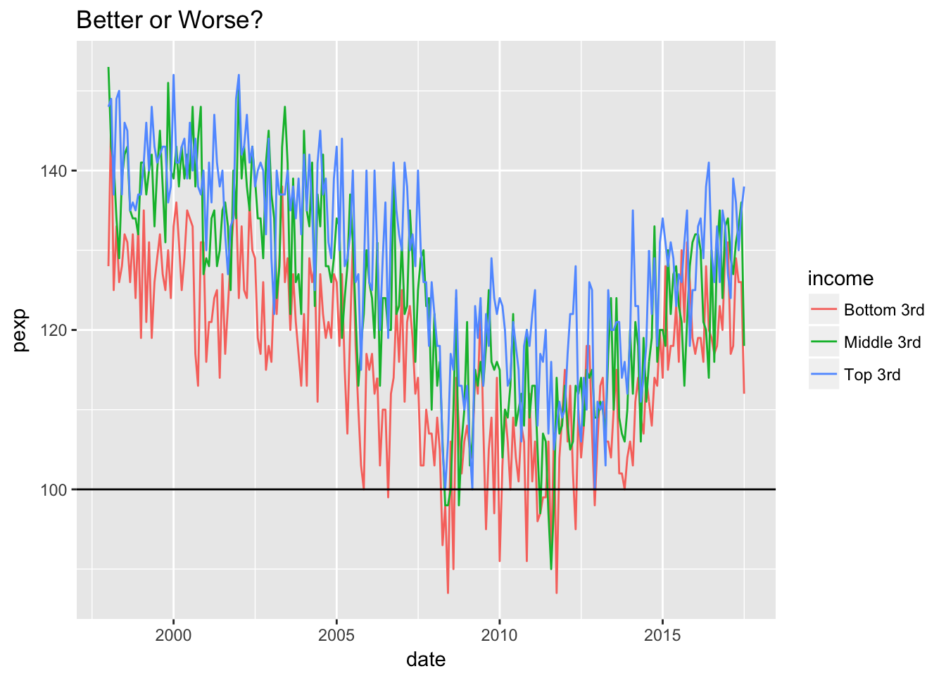
11.3 Stacked Periods
better <- ggplot(survey, aes(month, pexp, group = year, color = year)) +
  geom_line() +
  facet_wrap(~ income) +
  geom_hline(yintercept = 100) +
  ggtitle("Better or Worse?")
better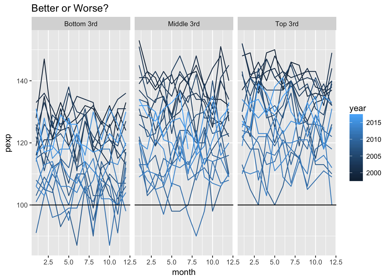
11.4 Polar Coordinates
better +
  coord_polar(theta = "x") +
  scale_x_continuous(breaks = c(1, 7), labels = month.name[c(1, 7)]) +
  theme_minimal()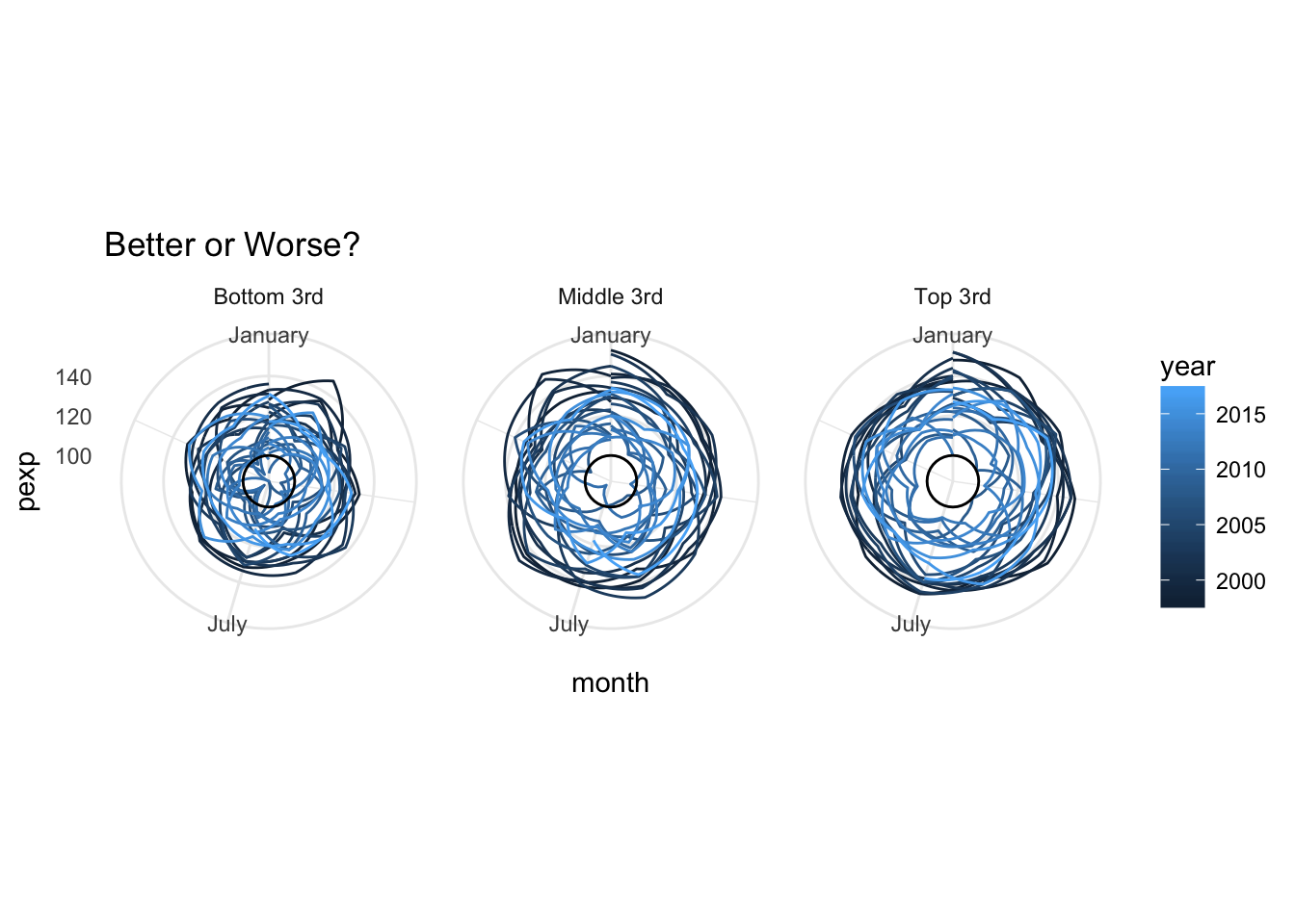
11.5 Assignment
Plot the other two variables (pjob and umex) in polar coordinates giving each plot a title that helps communicate the meaning of their respective variable.
11.6 Data Attribution
Source: Survey of Consumer Expectations, © 2013-2017 Federal Reserve Bank of New York (FRBNY). The SCE data are available without charge at /microeconomics/sce and may be used subject to license terms posted below. FRBNY disclaims any responsibility or legal liability for this analysis and interpretation of Survey of Consumer Expectations data.