Lecture 9 Jitter, Rug, and Aesthetics
9.1 Data
The Panel Study of Income Dynamics (PSID) is the longest running longitudinal household survey in the world.
From the Data page, you can use the Data Center to create customized datasets. We’ll use the Packaged Data option. Click the Main and Supplemental Studies link. Under the Supplemental Studies > Transition into Adulthood Supplement section, select the download for 2015.
To download the supplement you will need to sign in or register for a new account (by clicking the “New User?” link). Once you have logged in you should be able to download the zip file:
- ta2015.zip
9.1.1 Codebook
The TA2015_codebook.pdf is the perfect place for us to identify some key variables of interest. The following is an excerpt listing the variables we will use:
TA150003  "2015 PSID FAMILY IW (ID) NUMBER"
2015 PSID Family Interview Number

TA150004  "2015 INDIVIDUAL SEQUENCE NUMBER"
2015 PSID Sequence Number
This variable provides a means of identifying an individual's status with regard to the
PSID family unit at the time of the 2015 PSID interview.

Value/Range   Code Value/Range Text
1 - 20        Individuals in the family at the time of the 2015 PSID
              interview
51 - 59       Individuals in institutions at the time of the 2015 PSID
              interview

TA150005 "CURRENT STATE"
Current State (FIPS state codes)

TA150015 "A1_1 HOW SATISFIED W/ LIFE AS A WHOLE"
A1_1. We'd like to start by asking you about life in general. Please think about your
life-as-a-whole. How satisfied are you with it? Are you completely satisfied, very
satisfied, somewhat satisfied, not very satisfied, or not at all satisfied?

Value/Range   Code Value/Range Text
1             Completely satisfied
2             Very satisfied
3             Somewhat satisfied
4             Not very satisfied
5             Not at all satisfied
8             DK

TA150092 "D28A NUMBER OF CHILDREN"
D28a. How many (biological,) adopted, or step-children do you have?

TA150128 "E1 EMPLOYMENT STATUS 1ST MENTION"
E1. Now we have some questions about employment. We would like to know about what you do -
- are you working now, looking for work, keeping house, a student, or what?--1ST MENTION

Value/Range   Code Value/Range Text
1             Working now, including military
2             Only temporarily laid off; sick or maternity leave
3             Looking for work, unemployed
5             Disabled, permanently or temporarily
6             Keeping house
7             Student

TA150512 "F1 HOW MUCH EARN LAST YEAR"
F1. We try to understand how people all over the country are getting along financially, so
now I have some questions about earnings and income. How much did you earn altogether
from work in 2014, that is, before anything was deducted for taxes or other things,
including any income from bonuses, overtime, tips, commissions, military pay or any other
source?

Value/Range     Code Value/Range Text
0 - 5,000,000   Actual amount
    9,999,998   DK
    9,999,999   NA; refused
9.1.1.1 FIPS
In preparation for working with these variables, we can setup arrays to take the place of the codebook. The tigris package will give us the FIPS codes for each state:
install.packages(tigris)library(tidyverse)
state_fips <- tigris::fips_codes %>%
group_by(state) %>%
summarize(fips = as.numeric(first(state_code)))
fips2state <- array()
fips2state[state_fips$fips] <- state_fips$state
fips2state## [1] "AL" "AK" NA "AZ" "AR" "CA" NA "CO" "CT" "DE" "DC" "FL" "GA" NA
## [15] "HI" "ID" "IL" "IN" "IA" "KS" "KY" "LA" "ME" "MD" "MA" "MI" "MN" "MS"
## [29] "MO" "MT" "NE" "NV" "NH" "NJ" "NM" "NY" "NC" "ND" "OH" "OK" "OR" "PA"
## [43] NA "RI" "SC" "SD" "TN" "TX" "UT" "VT" "VA" NA "WA" "WV" "WI" "WY"
## [57] NA NA NA "AS" NA NA NA NA NA "GU" NA NA "MP" NA
## [71] NA "PR" NA "UM" NA NA NA "VI"9.1.1.2 Satisfaction
satisfaction <- array()
satisfaction_levels <- c("Completely satisfied", "Very satisfied", "Somewhat satisfied", "Not very satisfied", "Not at all satisfied", "DK")
satisfaction[c(1, 2, 3, 4, 5, 8)] <- satisfaction_levels
satisfaction
## [1] "Completely satisfied" "Very satisfied" "Somewhat satisfied"
## [4] "Not very satisfied" "Not at all satisfied" NA
## [7] NA "DK"9.1.1.3 Employment Status
We can also specify the array elements one by one:
employment <- array()
employment[1] <- "Working now, including military"
employment[2] <- "Only temporarily laid off; sick or maternity leave"
employment[3] <- "Looking for work, unemployed"
employment[5] <- "Disabled, permanently or temporarily"
employment[6] <- "Keeping house"
employment[7] <- "Student"
employment
## [1] "Working now, including military"
## [2] "Only temporarily laid off; sick or maternity leave"
## [3] "Looking for work, unemployed"
## [4] NA
## [5] "Disabled, permanently or temporarily"
## [6] "Keeping house"
## [7] "Student"9.1.2 Preprocessing the SPSS File
If you don’t have them already, open the zip file and move the TA2015.txt and TA2015.sps files into the data folder. For our import to work, We need to find a line that needs to be removed from the top of the sps file. The line we want to remove should look like the following line:
FILE HANDLE PSID / NAME = '[PATH]\TA2015.TXT' LRECL = 2173 .To find this line we can output the first 20 lines of the TA2015.sps file:
readLines("data/TA2015.sps", n = 10)## [1] ""
## [2] "**************************************************************************"
## [3] " Label : Transition to Adulthood Study 2015"
## [4] " Rows : 1641"
## [5] " Columns : 1304"
## [6] " ASCII File Date : July 5, 2017"
## [7] "*************************************************************************."
## [8] ""
## [9] "FILE HANDLE PSID / NAME = '[PATH]\\TA2015.TXT' LRECL = 2173 ."
## [10] "DATA LIST FILE = PSID FIXED /"Now we know the line to remove is line number 9, we can write a new file to be used in the processing step below.
input <- file("data/TA2015.sps")
output <- file("data/TA2015_clean.sps")

open(input, type = "r")
open(output, open = "w")

writeLines(readLines(input, n = 8), output)
invisible(readLines(input, n = 1))
writeLines(readLines(input), output)

close(input)
close(output)

readLines("data/TA2015_clean.sps", n = 10)
## [1] ""
## [2] "**************************************************************************"
## [3] " Label : Transition to Adulthood Study 2015"
## [4] " Rows : 1641"
## [5] " Columns : 1304"
## [6] " ASCII File Date : July 5, 2017"
## [7] "*************************************************************************."
## [8] ""
## [9] "DATA LIST FILE = PSID FIXED /"
## [10] " TA150001 1 - 1 TA150002 2 - 6 TA150003 7 - 11 "9.1.3 Importing with the SPSS file using memisc
The memisc package has useful tools for importing SPSS and Stata files that augment what already exists in base. Unfortunately, one of its dependencies, MASS, will mask the select method from dplyr. To avoid this, instead of loading memisc with library(memisc), we can prefix all memisc functions with memisc::.
install.packages("memisc")ta_importer <- memisc::spss.fixed.file("data/TA2015.txt", columns.file = "data/TA2015_clean.sps", varlab.file = "data/TA2015_clean.sps", to.lower = FALSE)
ta_full <- memisc::as.data.set(ta_importer)
ta_full##
## Data set with 1641 observations and 1304 variables
##
## TA150001 TA150002 TA150003 TA150004 TA150005 TA150006 TA150007 ...
## 1 1 1 4893 1 37 55 9 ...
## 2 1 2 2967 1 48 57 9 ...
## 3 1 3 6095 5 37 96 9 ...
## 4 1 4 3738 3 8 98 9 ...
## 5 1 5 6741 3 16 104 9 ...
## 6 1 6 4839 1 28 68 9 ...
## 7 1 7 3828 1 48 67 9 ...
## 8 1 8 5640 51 21 88 9 ...
## 9 1 9 5210 52 6 80 9 ...
## 10 1 10 339 3 18 93 9 ...
## 11 1 11 3192 2 26 66 9 ...
## 12 1 12 561 2 26 91 9 ...
## 13 1 13 2500 51 13 100 9 ...
## 14 1 14 5283 2 39 68 9 ...
## 15 1 15 6679 1 24 62 9 ...
## 16 1 16 3286 2 8 67 9 ...
## 17 1 17 3266 2 6 155 9 ...
## 18 1 18 3720 2 48 61 9 ...
## 19 1 19 3714 2 48 82 9 ...
## 20 1 20 6244 1 48 89 9 ...
## 21 1 21 4199 1 13 80 9 ...
## 22 1 22 3962 2 51 86 9 ...
## 23 1 23 2878 1 41 85 9 ...
## 24 1 24 3835 1 37 85 9 ...
## 25 1 25 487 51 13 91 9 ...
## .. ........ ........ ........ ........ ........ ........ ........ ...
## (25 of 1641 observations shown)9.1.4 Transform Data
Take the arrays we created above to process the file down to the variables we selected.
ta <- ta_full %>%
  as.data.frame() %>%
  as.tbl() %>%
  filter(TA150005 > 0) %>% # get rid of the 1 non-US response
  transmute(
    family_id         = TA150003,
    in_institution    = TA150004 > 50,
    state             = fips2state[TA150005],
    life_satisfaction = factor(satisfaction[TA150015], levels = satisfaction_levels, ordered = TRUE),
    children          = TA150092,
    employment_status = employment[TA150128],
    annual_earnings   = TA150512 %>% na_if(9999999) %>% na_if(9999999)
  )
ta
## # A tibble: 1,640 x 7
## family_id in_institution state life_satisfaction children
## <dbl> <lgl> <chr> <ord> <dbl>
## 1 4893 FALSE NC Somewhat satisfied 0
## 2 2967 FALSE TX Somewhat satisfied 0
## 3 6095 FALSE NC Somewhat satisfied 0
## 4 3738 FALSE CO Somewhat satisfied 0
## 5 6741 FALSE ID Very satisfied 0
## 6 4839 FALSE MS Completely satisfied 1
## 7 3828 FALSE TX Somewhat satisfied 0
## 8 5640 TRUE KY Completely satisfied 0
## 9 5210 TRUE CA Very satisfied 0
## 10 339 FALSE IN Somewhat satisfied 0
## # ... with 1,630 more rows, and 2 more variables: employment_status <chr>,
## # annual_earnings <dbl>library(ggplot2)
base_plot <- ggplot(ta, aes(life_satisfaction, annual_earnings)) + scale_y_log10()
base_plot + geom_point()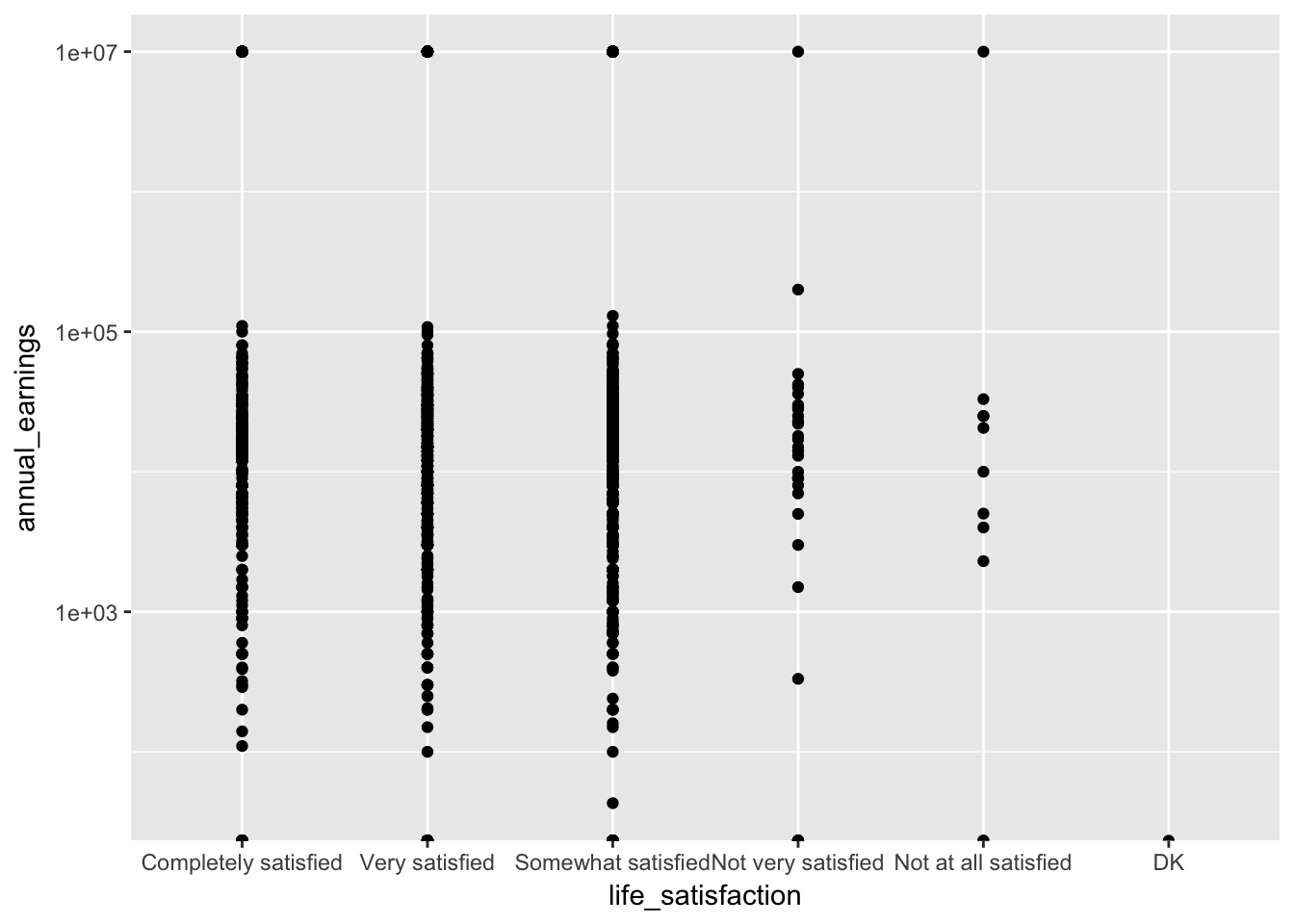
9.2 Jitter
When many points overlap, using geom_jitter adjusts the position of each point to minimize overlap.
base_plot + geom_jitter()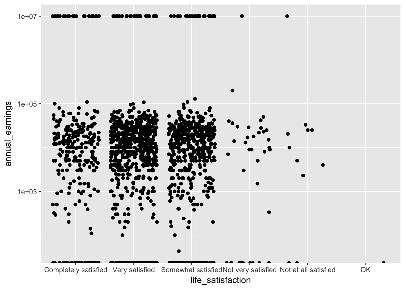
See how this compares to using alpha (i.e., opacity) to see how many points are in a given position:
base_plot + geom_point(alpha = 0.1)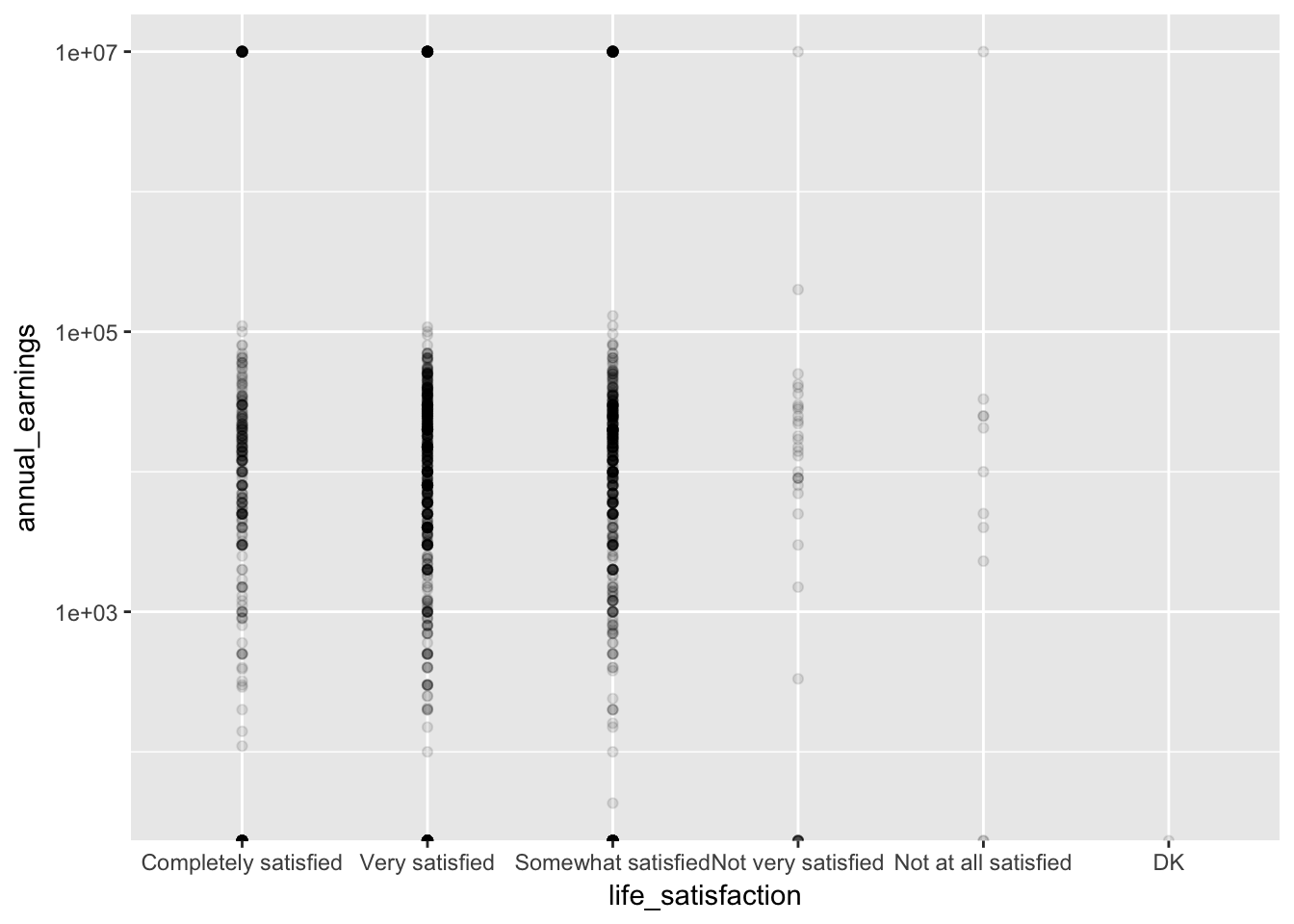
9.3 Rug
Often when there are many points, we want to plot a summary that presents the general shape of the data.
base_plot + geom_violin()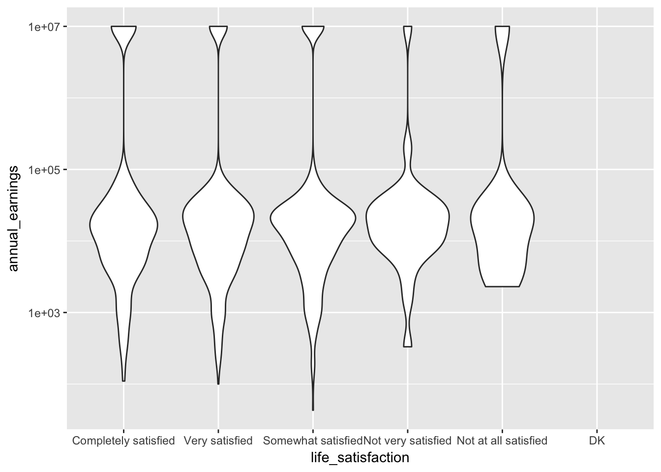
The geom_rug gives us a rug plot that we can use to highlight where actual observations occured when we create these summary plots.
base_plot + geom_violin() + geom_rug()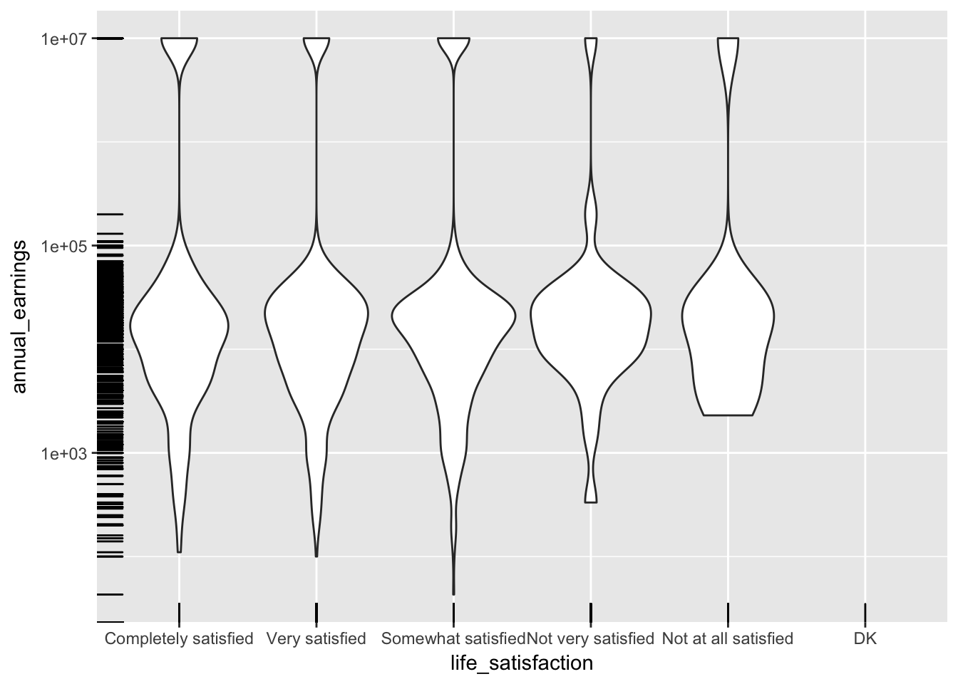
Both alpha and jitter can be applied to the rug as well.
base_plot + geom_violin() + geom_rug(alpha = 0.1, position = "jitter")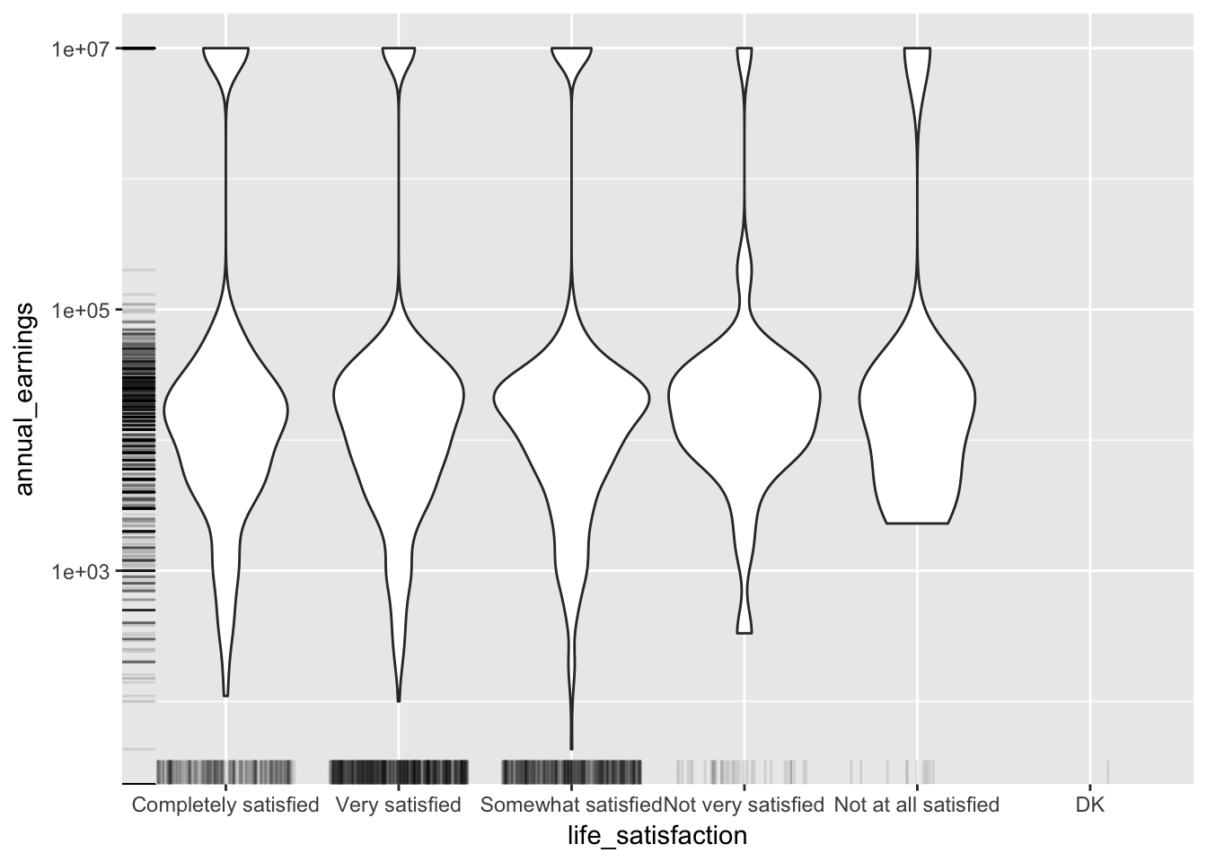
Now we can see that rug did in fact create a line on the x-axis for each observation. We can use the sides property to only display the rug on the left and right ("lr")
base_plot + geom_violin() + geom_rug(alpha = 0.1, position = "jitter", sides = "lr")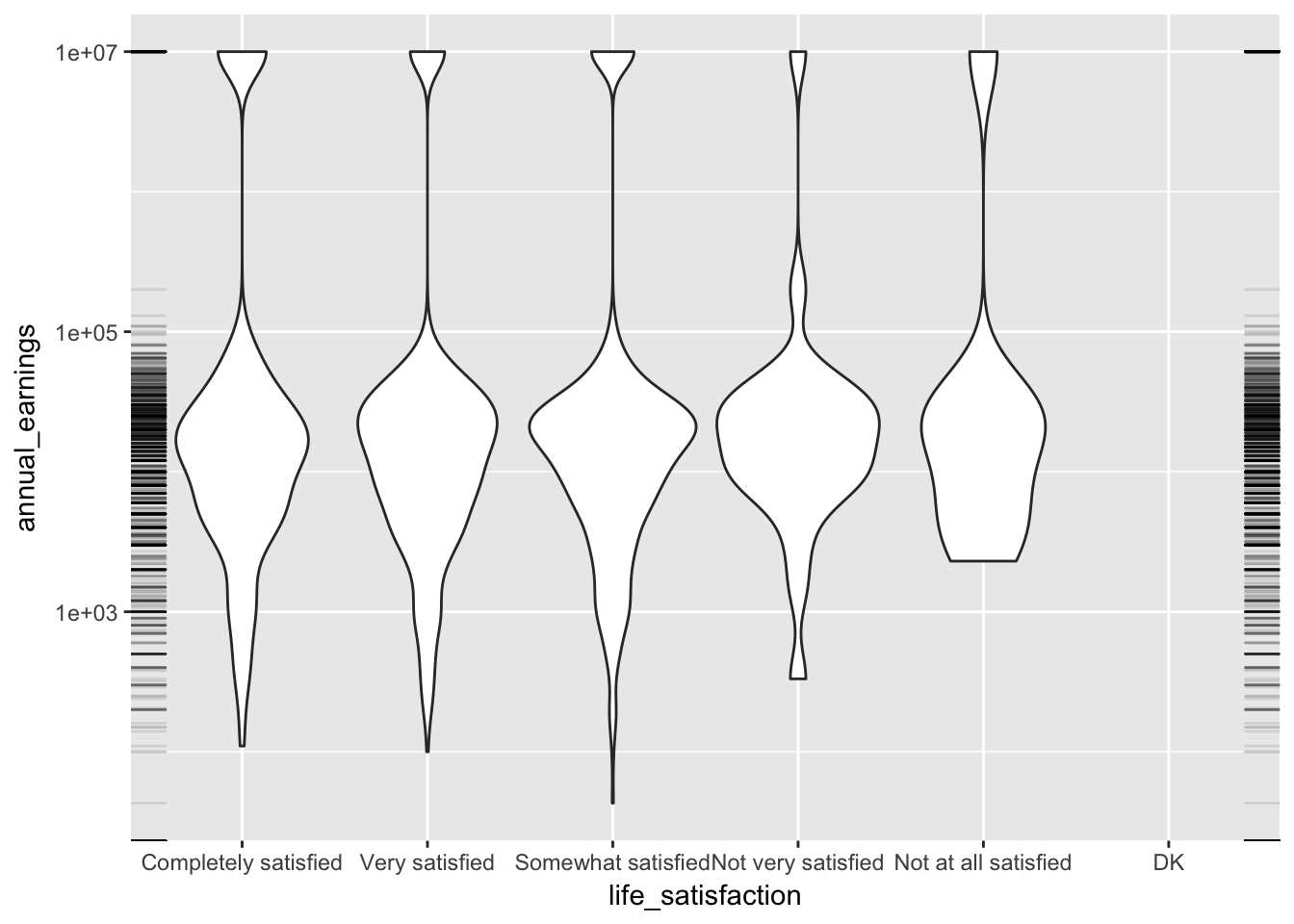
9.4 Aesthetics
Aesthetics are the visual properties that define each graph. In ggplot, the aes() function is used to create a mapping from your data to these visual properties. We most often use aes() to map our variables to the x and y dimension. Above, we used the fact that the first two arguments to aes() are x and y. That is,
aes(x = life_satisfaction, y = annual_earnings)gives the same result as
aes(life_satisfaction, annual_earnings)Anytime we want more than two dimensions of our data displayed, it’s useful to map the extra variables to other features of our graph (e.g., size, color, alpha, etc.). Let’s add number of children to our graph assigning children to color. (In ggplot both American and British spellings are supported, so you can use color or colour.)
ggplot(ta, aes(life_satisfaction, annual_earnings, color = children)) +
  scale_y_log10() +
  geom_jitter()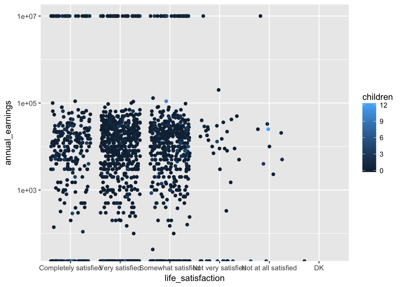
If the children variable was a factor, more distinct colors would have been chosen. We can see this by coloring by employment_status instead.
ggplot(ta, aes(life_satisfaction, annual_earnings, color = employment_status)) +
  scale_y_log10() +
  geom_jitter()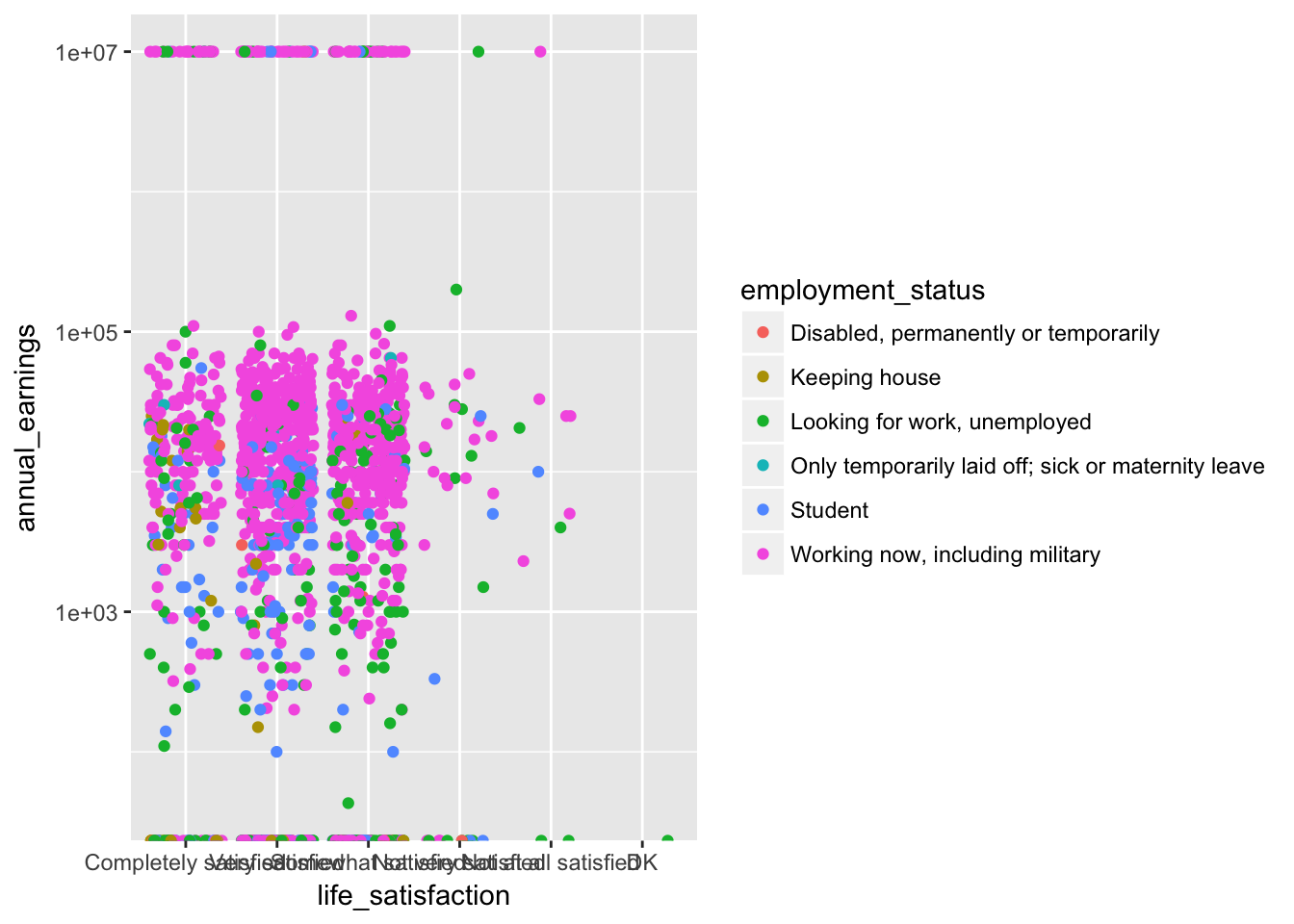
You can emphasize a variable by encoding in more than one visual aesthetic. Let’s map children to color, size, and alpha.
ggplot(ta, aes(life_satisfaction, annual_earnings, color = children, size = children, alpha = children)) +
  scale_y_log10("Annual Earnings", labels = scales::dollar) +
  geom_jitter()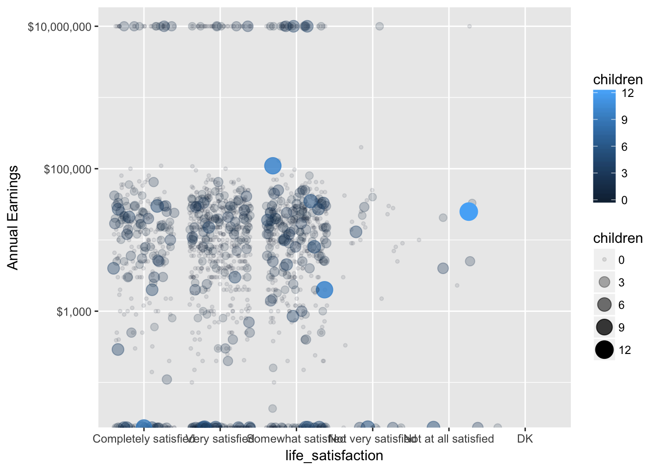
9.5 Assignment
Open the codebook (data/TA2015_codebook.pdf) and search for two new variables to visualize. Create a plot that makes use of both jitter and rug.